qtl2shiny Developer Guide

This document is a Developer Guide for the R/qtl2shiny package, with goals to explain:

data structures and folder organization
package workflow and shiny tool components

library(qtl2shiny)

Those wishing to use the shiny interface with their own data will want to read about the data structures, or contact me. Those wishing to extend capabilities of the package, or understand its inner working, will be interested in the package organization. This developer guide was generated with the help of Antigravity, with significant editing and rewriting; see Create Developer’s Guide to qtl2shiny.

Data Structures and Folder Organization

The interface assumes the Shiny app file app.R is in a directory with other support documents and the data folder, qtl2shinyData. There is no need to change this file; just put it in place.

The CSV file projects.csv, in the sub-folder, qtl2shinyData, contains project information. This file has the following content:

project,taxa,directory
Recla,CCmouse,qtl2shinyData

The column names are fixed. The project is the project name (Recla), taxa has the taxa name (CCmouse), and directory is the relative or absolute address of the directory where data are kept (qtl2shinyData, which is relative here). In this case, the basic structure of the app is:

app.R
about.md
about-extended.md
qtl2shinyData/
qtl2shinyData/projects.csv
qtl2shinyData/CCmouse/
qtl2shinyData/CCmouse/Recla/

The about.md and about-extended.md files are place-holders for now for online documentation. All data may be stored under the directory (qtl2shinyData).

Detailed information about the taxa and project can be found with the CCmouse.Rmd and Recla.Rmd examples, respectively.

Taxa information

The taxa sub-directory (CCmouse) contains the following files. See https://github.com/rqtl/qtl2db for explanation of the SQL databases and query routines.

file	contents
`allele_info.rds`	information on alleles for taxa
`taxa_info.rds`	information on taxa (name of species for Ensembl lookup)
`cc-variants.sqlite`	CC structural variants in SQL database
`mouse_genes_mgi.sqlite`	mouse genes curated by MGI in SQL database
`query_genes.rds`	query routine for genes
`query_variants.rds`	query routines for structural variants

Project Information

The project sub-sub-directory (Recla) has the data specific to the project. An example of how this is created can be found in Recla.Rmd. Most of the objects are stored as RDS. The genotype probabilities are converted from calc_genoprob to fst_genoprob format using R/qtl2fst. Query routines are somewhat analogous to those used for taxa above.

Note that R/qtl2 wants data files to be consistent in terms of individual identifiers. The covar.rds and pheno_data.rds files have identifiers as row names, which are also used in the genotype probabilities.

file	contents
`genoprob/`	directory with genotype probabilities created with R/qtl2fst
`kinship.rds`	kinship object using LOCO (see R/qtl2)
`pmap.rds`	physical map
`covar.rds`	data frame of covariates (row = individual, column = covariate)
`pheno_data.rds`	matrix of phenotype data (row = individual, column = phenotype)
`analyses.rds`	data frame of information about analyses (one row per phenotype)
`peaks.rds`	data frame of peak information (one row per peak)
`hotspot.rds`	hotspot object with counts of peaks by position and phenotype set
`query_mrna.rds`	query of mRNA data
`query_probs.rds`	query of genotype probabilities

Likely changes:

pheno_data.rds may become a fst database
analyses.rds will be redesigned

Some projects have an RNAseq folder. This, and accompanying routines for mRNA now in R/qtl2pattern and other packages, will likely be redesigned. Currently, code is set up for only one type of mRNA data.

Data files

The easiest way to set up data files is to look at the example in Recla.Rmd. Once you have created the objects in R, you can save them as, for instance, RDS files (here using the same names as in Recla.Rmd).

project_info <- utils::read.csv("project.csv")
project_dir <- file.path(project_info$taxa[1],
                         project_info$project[1])
saveRDS(kinship, file.path(project_dir, "kinship.rds"))
saveRDS(pmap, file.path(project_dir, "pmap.rds"))
saveRDS(covar, file.path(project_dir, "covar.rds"))
saveRDS(pheno, file.path(project_dir, "pheno_data.rds"))
saveRDS(analyses_tbl, file.path(project_dir, "analyses.rds"))
saveRDS(peaks, file.path(project_dir, "peaks.rds"))
saveRDS(hots, file.path(project_dir, "hotspot.rds"))

Genotype probabilities

Genotype probabilities get stored in fst databases by chromosome for rapid access. This takes a few steps, starting with creating a directory to store files and calculating genotype probabilities for allele pairs.

# Create directory for fst data; must call it "genoprob"
fst_dir <- file.path(project_dir, "genoprob")
dir.create(fst_dir)

# Calculate allele pair genotype probabilities
probs <- qtl2::calc_genoprob(recla, gmap, err=0.002)
# Convert allele pair probs to fst via qtl2fst
fprobs <- qtl2pattern::fst_genoprob(probs, "probs", fst_dir)
saveRDS(fprobs, file = file.path(fst_dir, "fprobs.rds"))

# Compute allele genotype probabilities from those for allele pairs
aprobs <- genoprob_to_alleleprob(probs)
# Convert allele probs to fst via qtl2fst
faprobs <- fst_genoprob(aprobs, "aprobs", fst_dir)
saveRDS(faprobs, file = file.path(fst_dir, "faprobs.rds"))

Query files

The query files are designed to encapsulate specific information about where data are stored and how to retrieve them, so that different projects might use different strategies. For instance, some projects might use CSV or RDS files, while others might use SQL or fst databases. There are four query objects, for genes, variants, mrna and probs.

Note that if you use a similar format as CCmouse.Rmd and Recla.Rmd examples to create and store the queries, you may have to quit RStudio and restart it to have it properly pick up the project or taxa directory.

The following two create functions are in R/qtl2. They create functions (query_genes and query_variants) that contain, in their local environment, the location of the respective SQL database. Saving these as RDS preserves this environment information for later reuse.

query_genes <- 
  qtl2::create_gene_query_func("CCmouse/mouse_genes.sqlite")
saveRDS(query_genes, "query_genes.rds")

query_variants <- 
  qtl2::create_variant_query_func("CCmouse/cc_variants.sqlite"))
saveRDS(query_variants, "query_variants.rds")

This allows calls of the following form to be embedded in code, without reference to where the database is, or even what type of database it might be. Here we look on chromosome "1" between 39 and 40 Mbp.

genes <- query_genes("1", 39, 40)
variants <- query_variants("1", 39, 40)

The above two routines would generally be used across all projects involving the CC mouse. The following two routines are project specific, refering to genotype probabilities and mRNA data. They do not directly identify the data file, as that is currently hard-coded into the R/qtl2pattern package. These will change substantially in the near future.

query_probs <- qtl2pattern::create_probs_query_func_do("CCmouse/Recla")
saveRDS(query_probs, "query_probs.rds")

query_mrna <- qtl2pattern::create_mrna_query_func_do(NULL)
saveRDS(query_probs, "query_mrna.rds")

Again, these enable calls to access data in a region. The Recla data does not have mRNA data, but we still have to create a NULL query. I include additional arguments that are used for these routines. They call, respectively, qtl2pattern::read_probs and qtl2pattern::read_mrna (at least, when there are mRNA data).

probs <- query_probs("1", 39, 40, allele = TRUE, method = "fst")
mrna <- query_mrna("1", 39, 40, local = TRUE, qtl = FALSE)

Remote files and connections

It is possible for data for a taxa and project to be stored in another place, in which case an absolute address would be supplied in the projects.csv file. For efficient access, that absolute address should probably be in a filesystem that is locally accessible. However, it is possible to have a connection, such as a URL; this has not been tried yet.

File types

Most data files work well to be RDS, which preserve attributes of an R object. This is useful if some data columns should be interpreted as character or factor, for instance. Also, the query calls must be stored as RDS to preserve the calling environment.

Genotype probabilities are assumed to be fst databases. This ensures rapid access to this information, which is the largest set of data besides the SNP information.

Package Workflow and Shiny Tool Components

The qtl2shiny interface can be invoked within R using runApp on the file app.R. There is a routine qtl2shinyApp in the package to do this as well:

qtl2shiny::qtl2shinyApp

However, one first should set up the data and query files as described above.

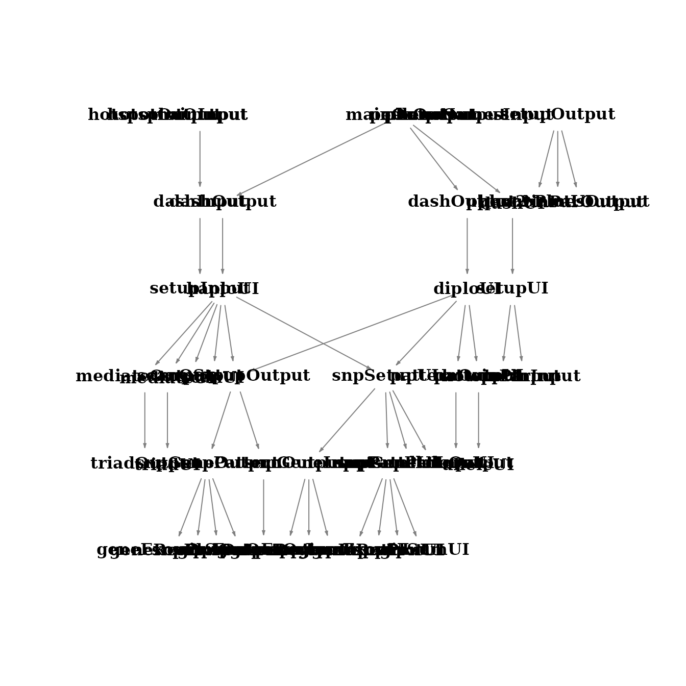
The shiny server consists of the server app (server() and ui() in file app.R) and 27 shiny modules. The modules form a directed acyclic graph with Main being the root node.

character(0)

character(0)


  1 
152

character(0)

 [38;5;246m# A tibble: 9 × 3 [39m
  logic    shiny        n
   [3m [38;5;246m<chr> [39m [23m     [3m [38;5;246m<chr> [39m [23m     [3m [38;5;246m<int> [39m [23m
 [38;5;250m1 [39m download download     2
 [38;5;250m2 [39m output   output      25
 [38;5;250m3 [39m reactive argument    20
 [38;5;250m4 [39m reactive input        7
 [38;5;250m5 [39m reactive result      12
 [38;5;250m6 [39m server   module      33
 [38;5;250m7 [39m shiny    shiny        1
 [38;5;250m8 [39m static   argument     1
 [38;5;250m9 [39m ui       module      51

 [38;5;246m# A tibble: 7 × 2 [39m
  assign       n
   [3m [38;5;246m<chr> [39m [23m     [3m [38;5;246m<int> [39m [23m
 [38;5;250m1 [39m argument   132
 [38;5;250m2 [39m download    19
 [38;5;250m3 [39m input        6
 [38;5;250m4 [39m output      26
 [38;5;250m5 [39m result      23
 [38;5;250m6 [39m server      31
 [38;5;250m7 [39m ui          45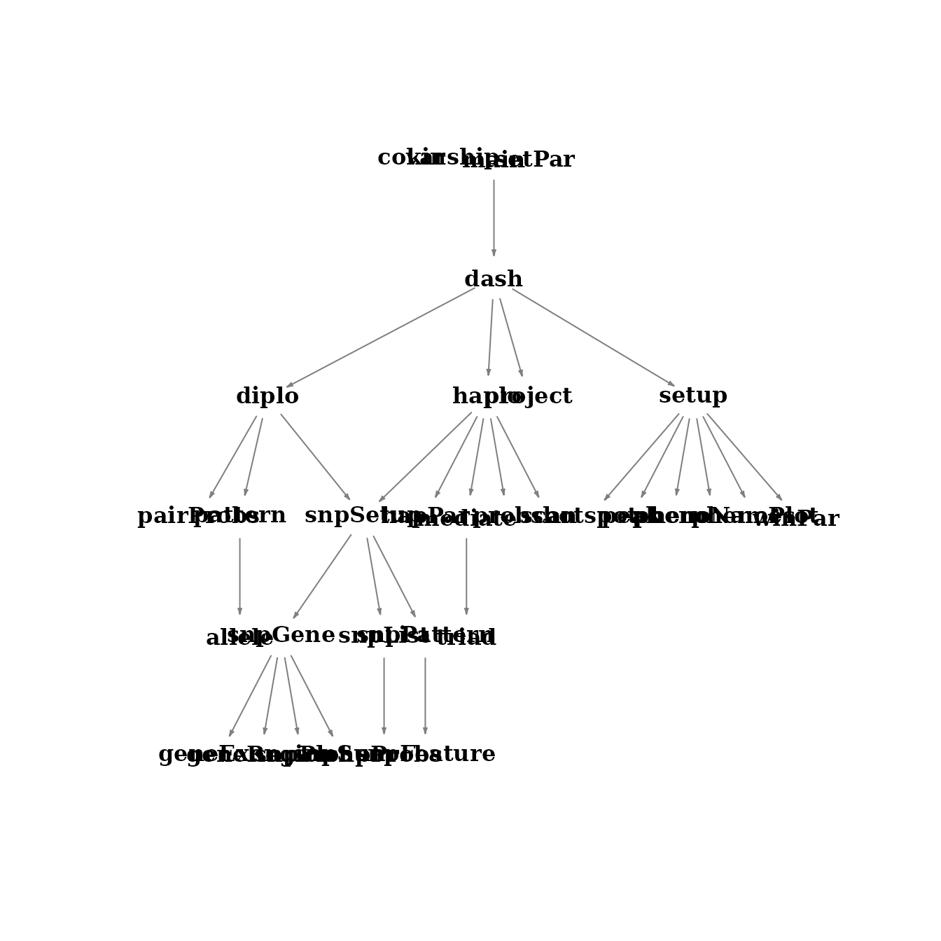

The Main module calls the Setup, Haplo and Diplo modules, corresponding to the three dashboard menu items. Each of these modules in turn calls other modules. The modules were each designed to do one task, and be kept small, ideally about 100 lines of code (including documentation). Here is a list of modules:

modeul	lines	task	output
`Main`	129	call Setup, Haplo, Diplo
`Setup`	209	set up project
`Haplo`	103	Haplotype Scans
`Diplo`	107	SNP/Gene Action

`Project`	47	pick project
`Peaks`	175	select chr, peak and window width
`Phenos`	88	phenotype information	table
`Hotspot`	190	hotspot count by location	plot, table
`PhenoPlot`	66	plot phenotypes	plot

`Probs`	93	allele genotype probabilities
`ScanCoef`	210	allele genome LOD and effect scans	plot, table
`Mediate`	306	mediation by other phenotypes	plot, table
`Scatter`	149	scatter plot for mediator	plot

`PairProbs`	93	allele pair genotype probabilities
`Pattern`	247	LOD and imputed SNP effects by pattern	plot, table
`Allele`	126	allele and allele pair means	plot, tablt

`SNPSetup`	225	set up SNP processng
`SNPPattern`	276	SNP allele patterns	plot, table
`SNPFeature`	113	top SNP features	plot, table
`SNPProbs`	93	SNP genotype probabilities
`SNPGene`	102	SNP & Gene Choice	table
`SNPPlot`	64	plot SNP association	plot
`SNPSum`	143	create table of top SNPs	table
`GeneRegion`	115	genes and SNPs in region	plot, table
`GeneExon`	162	exons for individual genes	plot, table

Brian S. Yandell

15 Jul 2026