List of scan1coef objects

Create a list of scan1coef objects using scan1coef.

Summary of object of class listof_scan1coef, which is a list of objects of class scan1coef.

Summary of object of class listof_scan1coef, which is a list of objects of class scan1coef.

Subset of object of class listof_scan1coef, which is a list of objects of class scan1coef.

Usage

listof_scan1coef(
  probs,
  phe,
  K = NULL,
  covar = NULL,
  blups = FALSE,
  center = FALSE,
  ...
)

summary_listof_scan1coef(
  object,
  scan1_object,
  map,
  coef_names = dimnames(object[[1]])[[2]],
  center = TRUE,
  ...
)

# S3 method for class 'listof_scan1coef'
summary(object, ...)

summary_scan1coef(object, scan1_object, map, ...)

# S3 method for class 'scan1coef'
summary(object, ...)

subset_listof_scan1coef(x, elements, ...)

# S3 method for class 'listof_scan1coef'
subset(x, ...)

# S3 method for class 'listof_scan1coef'
x[...]

Arguments

probs

genotype probabilities object for one chromosome from calc_genoprob

phe

data frame of phenotypes

K

list of length 1 with kinship matrix

covar

matrix of covariates

blups

Create BLUPs if TRUE

center

center coefficients if TRUE

...

ignored

object

object of class listof_scan1coef

scan1_object

object from scan1

map

A list of vectors of marker positions, as produced by insert_pseudomarkers.

coef_names

names of effect coefficients (default is all coefficient names)

x

object of class listof_scan1coef

elements

indexes or names of list elements in x

Value

object of class listof_scan1coef

Author

Brian S Yandell, brian.yandell@wisc.edu

Examples

# read data
iron <- qtl2::read_cross2(system.file("extdata", "iron.zip", package="qtl2"))

# insert pseudomarkers into map
map <- qtl2::insert_pseudomarkers(iron$gmap, step=1)

# calculate genotype probabilities
probs <- qtl2::calc_genoprob(iron, map, error_prob=0.002)

# Ensure that covariates have names attribute
covar <- match(iron$covar$sex, c("f", "m")) # make numeric
names(covar) <- rownames(iron$covar)

# Calculate scan1coef on all phenotypes,
# returning a list of \code{\link[qtl2]{scan1coef}} objects
out <- listof_scan1coef(probs[,7], iron$pheno, addcovar = covar, center = TRUE)

# Plot coefficients for all phenotypes
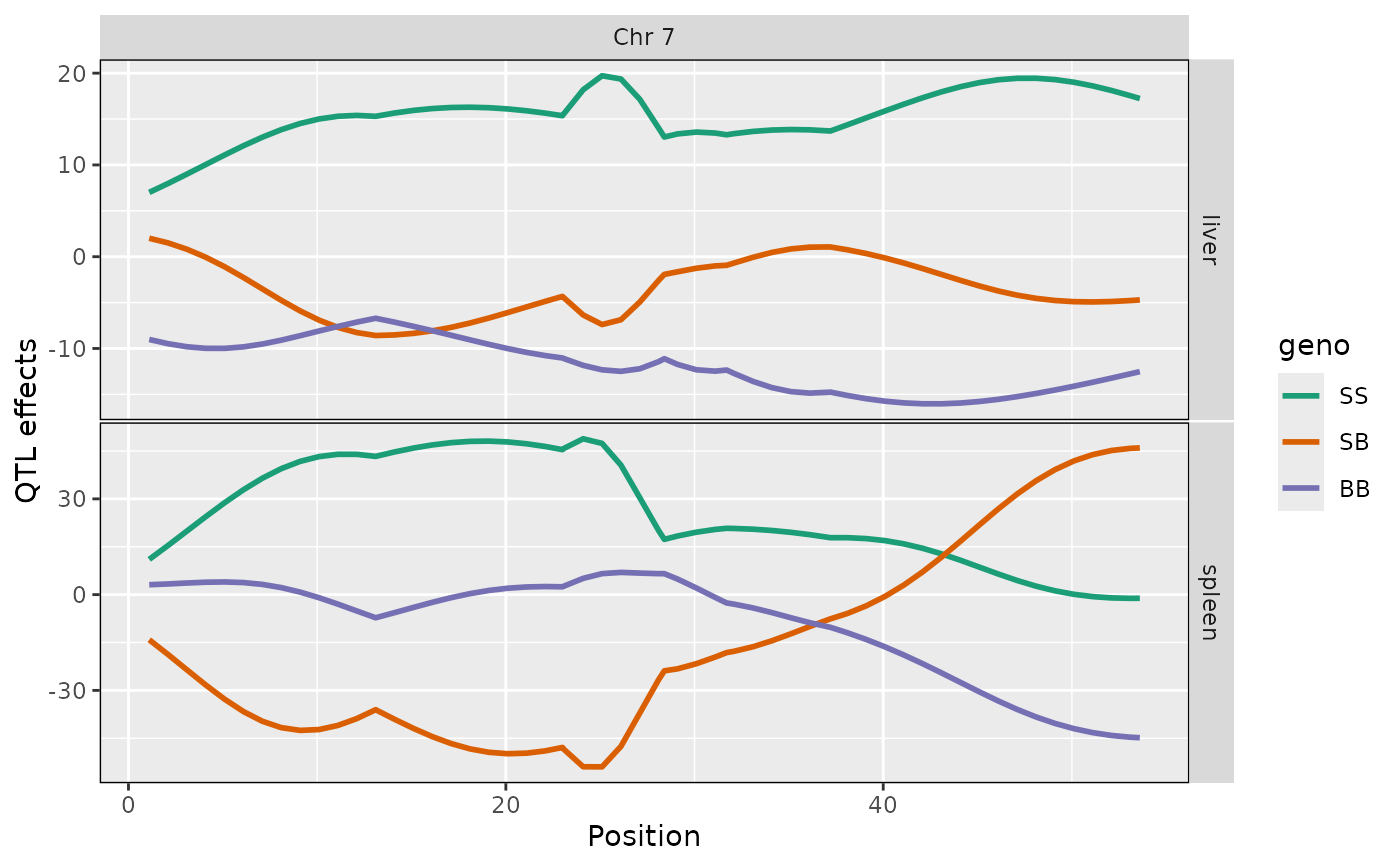
ggplot2::autoplot(out, map[7], columns = 1:3)


# Summary of coefficients at scan peak
scan_pr <- qtl2::scan1(probs[,7], iron$pheno)
summary(out, scan_pr, map[7])
#> # A tibble: 2 × 10
#>   pheno  chr     pos marker     lod     SS    SB     BB    ac1 intercept
#>   <chr>  <fct> <dbl> <chr>    <dbl>  <dbl> <dbl>  <dbl>  <dbl>     <dbl>
#> 1 liver  7      50.1 c7.loc50  4.05  -3.57 -27.5  -36.7  -55.3      123.
#> 2 spleen 7      53.6 D7Mit71   1.34 -91.0  -43.8 -135.  -197.       466.